The goal of statistics

Usually, we do not have the luxury of
getting access to the full
population of what we want to study.
We have to rely on a sample (from this
population) to make inferences
about the characteristics of the full population.
Null Hypothesis Significance Testing
Could my observed statistic ($\overset{\hat{}}{p}$, $\bar{x}$) be coming from a population centered at a certain value of parameter ($\pi$, $\mu$)?
What would the distribution of samples statistics ($\overset{\hat{}}{p}$, $\bar{x}$) coming from this hypothesized population look like? What is the probability of my observed statistic happening in this distribution ?
Resampling:
Let's simulate it and see (no assumption)
Theory:
- For a proportion, it's a normal distribution centered at
$\pi$, and with a standard deviation of $\sqrt{\frac{\pi(1-\pi)}{n}}$
- For a mean, it's a $t$-distribution centered at
$\mu$, and with a standard deviation of $\frac{\sigma}{\sqrt{n}}$ (but use $\frac{s}{\sqrt{n}}$ instead).
Null Hypothesis Significance Testing
Resampling
Theory
Confidence intervals
What would be a range of statistics values ($\overset{\hat{}}{p}$, $\bar{x}$) I am confident will contain the true value parameter ($\pi$, $\mu$) for the population my sample is coming from?
What would be a possible range of statistics ($\overset{\hat{}}{p}$, $\bar{x}$) I would
obtain if I had access to other samples from this same distribution?
Resampling:
Let's use our data and draw lots of Bootstrap samples.
We will keep the center $95\%$ values as the range of values we are confident is containing the true value
of the parameter of the population our sample is coming from.
Theory:
We will consider a range of values centered at our
observed statistic and of width $\pm2SE$ on each
side.
$SE=\sqrt{\frac{\overset{\hat{}}{p}(1-\overset{\hat{}}{p})}{n}}$ for a sample proportion
$SE=\frac{s}{\sqrt{n}}$ for a sample mean
Confidence intervals
Resampling
Theory
NHST vs Confidence intervals
Null Hypothesis testing
Confidence intervals (95%)
Could my observed statistic ($\overset{\hat{}}{p}$, $\bar{x}$) be coming from a population centered at a certain value of parameter [$\pi$, $\mu$]?
What would be a range of values I am confident will contain the true value of the population parameter my sample is coming from?
What would the distribution of samples statistics coming from this hypothesized population look like? What is the probability of my observed statistic happening in this distribution ?
What would be a possible range of statistics I would
obtain if I had access to other samples from this same distribution? The central $95\%$ of this interval is very
likely to contain the parameter value of the distribution
my sample is coming from.
NHST vs Confidence intervals
NHST
95% CI
Statistics in the Courtroom: United States v. Kristen Gilbert
Kristen Gilbert is a former nurse and an American serial killer who was convicted of four murders and two attempted murders of patients admitted to the Veterans Affairs Medical Center (VAMC) in Northampton, Massachusetts.
She induced cardiac arrest in patients by injecting their intravenous therapy bags with massive doses of epinephrine, an untraceable heart stimulant.
She would then respond to the coded emergency, often resuscitating the patients herself.
Deaths in the medical ward
The graph shows data from the VA hospital where Kristen Gilbert worked. Each set of three bars shows one year’s worth of data, starting in 1988, and running through 1997.
Gilbert's shifts
1990:
Night
1991-1996:
Evening
Data at the Gilbert's trial
Part of the evidence presented against Gilbert at her murder trial was a statistical analysis of the 8-shift records for the eighteen months leading up to the end of February, 1996. (That February was the month when Gilbert’s coworkers met with their supervisor to express their concerns; shortly after that, Gilbert took a medical leave.)
With 547 days during the period in question, and three shifts per day, there were 1641 shifts in all. Out of these 1641 shifts, there were 74 for which there was at least one death.
What are the observational units?
The 1641 8h-shifts (one 8h-shift is one observational unit)
What are the variables? What type are they?
Response variable: was there at least one death during the shift?
Explanatory variable: was Gilbert working or not during the shift?
Explanatory & Response variables
A response variable is the variable about which questions are asked; it measures the outcome of the study.
An explanatory variable is any factor that can influence, explain or predict the response variable.
The response variable is usually called dependent, while the explanatory variable is sometimes called independent.
Two-way tables
A two-way table is used to show the relationship between two categorical variables. The categories for one variable are listed down the side (rows) and the categories for the second variable are listed across the top (columns). Each cell of the table contains the count of the number of data cases that are in both the row and column categories.
Note: It is often helpful to also include the totals (both for rows and columns) in the margins of a two-way table.
Response variable
Explanatory variable
| Death on shift? |
Gilbert present? | ||
| Yes | No | Total | |
| Yes | 40 | 34 | 74 |
| No | 217 | 1350 | 1567 |
| Total | 257 | 1384 | 1641 |
Deaths pattern during the 8h-shifts
| Death on shift? |
Gilbert present? | ||
| Yes | No | Total | |
| Yes | 40 | 34 | 74 |
| No | 217 | 1350 | 1567 |
| Total | 257 | 1384 | 1641 |
Normalizing the data
To take into account the sample sizes into your data, it is much more useful to look at the conditional proportions of your response variable, where we compute the proportion of "positive" responses separately within each explanatory variable group.
Raw data
Conditional proportions
| Death on shift? |
Gilbert present? | ||
| Yes | No | Total | |
| Yes | 40 | 34 | 74 |
| No | 217 | 1350 | 1567 |
| Total | 257 | 1384 | 1641 |
| Death on shift? |
Gilbert present? | |
| Yes | No | |
| Yes | 0.156 | 0.025 |
| No | 0.844 | 0.975 |
| Total | 1 | 1 |
Normalizing the data
Raw data
Conditional proportions
The goal of our study is to see whether we can find an association between the presence of Gilbert
during a shift and the proportion of shifts for which at least a death occured.
=> how do the two conditional proportions compare?
Comparing 2 proportions
| Death on shift? |
Gilbert present? | |
| Yes | No | |
| Yes | 0.156 | 0.025 |
| No | 0.844 | 0.975 |
| Total | 1 | 1 |
Arithmetic difference in the conditional proportions of shifts with deaths:
$d=\overset{\hat{}}{p}_{\textrm{present}}-\overset{\hat{}}{p}_{\textrm{absent}}$
$d=0.156-0.025=0.131$
Conditional proportions
Calculating the relative risk
The relative risk is the ratio of two conditional proportions. It indicates how many times greater the risk of an outcome is for one group compared to another.
| Death on shift? |
Gilbert present? | |
| Yes | No | |
| Yes | 0.156 | 0.025 |
| No | 0.844 | 0.975 |
| Total | 1 | 1 |
Relative risk:
What does it mean?
It is 6.24 times more likely to observe at least one death
during a shift in which Gilbert is present
Can we find an association?
This difference of 13.1% between the conditional proportions (or similarly, the relative risk of 6.24), appears quite substantial.
We are interested in investigating whether the presence of
Gilbert during a shift is associated with a higher proportion
of death occurrence.
Alternative hypothesis:
A death is more likely to occur in a shift in which Gilbert
is present
($d>0$ or $RR>1$).
What is the null hypothesis in this investigation?
A death is as likely to occur in a shift in which Gilbert
is present or not ($d=0$ or
$RR=1$).
The observed difference in relative proportion of death occurrence (or the high RR) could be explained by chance alone.
Simulating the null
Our strategy will be to determine how surprising the observed result would be if the null hypothesis were true . We can determine this by using simulation to generate a large number of "could have been" results under that null hypothesis and examine the null distribution of our statistic.
If the observed result from our investigation falls in the tail of that distribution, then we have strong evidence against the null hypothesis.
Simulating the null
One possible choice of statistic for comparing these
two groups is the difference in the observed sample proportion of shifts for which a death was recorded. (The RR would have been valid too)
$\overset{\hat{}}{p}_{\textrm{present}}-\overset{\hat{}}{p}_{\textrm{absent}}=0.131$.
In the actual data, there were 74 shifts for which at least
one death occurred. If there was no association of death
with the explanatory variable (presence or not of Gilbert in
the shift), then those deaths would have occurred regardless
of whether or not Gilbert was present during the shift.
=> if this is true, then any differences we do see between
the two groups arise solely from the randomness in the
assignment to the explanatory variable groups.
Simulating the null
To evaluate the statistical significance of the observed difference in our groups ($\overset{\hat{}}{p}_{\textrm{present}}-\overset{\hat{}}{p}_{\textrm{absent}}=0.131$), we will investigate how large the difference in conditional proportion tends to be just from the random assignment of outcomes (death or not) to the explanatory variable groups.
Think of this simulation as a simulation with colored balls.
74 yellow balls
1567 blue balls
We will simulate the random assignment process of the shifts to the two groups by shuffling the balls and putting
257 in one bucket and 1384 in another bucket.
| Death on shift? |
Gilbert present? | ||
| Yes | No | Total | |
| Yes | 40 | 34 | 74 |
| No | 217 | 1350 | 1567 |
| Total | 257 | 1384 | 1641 |
Simulating the null
We perform this simulation 10000 times, so at the end
we obtain
10000 differences of the conditional proportions between the 2 groups.
=> 10 000 differences $\overset{\hat{}}{p}_{\textrm{1}}-\overset{\hat{}}{p}_{\textrm{2}}$ that we could have observed if the presence or absence of Gilbert during a shift
did not play a role in the likelihood of observing a death
during the shift.
Simulating the null
Theory: two-sample z-test
According to theory the distribution of the differences in sample conditional proportions will be normal, centered at $0$, with a standard deviation of $\sqrt{\overset{\hat{}}{p}(1-\overset{\hat{}}{p})(\frac{1}{n_1}+\frac{1}{n_2})}$ where $\overset{\hat{}}{p}$ is the overall proportion of successes for the two groups combined (total number of successes divided by the total sample size)
A $z$ statistic can then be calculated using:
$z=\frac{\textrm{observed statistic}-\textrm{hypothesized value}}{\textrm{standard error of statistic}}$
$z=\frac{(\overset{\hat{}}{p}_1-\overset{\hat{}}{p}_2)-0}{\sqrt{\overset{\hat{}}{p}(1-\overset{\hat{}}{p})(\frac{1}{n_1}+\frac{1}{n_2})}} =\frac{\overset{\hat{}}{p}_1-\overset{\hat{}}{p}_2}{\sqrt{\overset{\hat{}}{p}(1-\overset{\hat{}}{p})(\frac{1}{n_1}+\frac{1}{n_2})}}$
Theory: two-sample z-test
where $\overset{\hat{}}{p}$ is the overall proportion of successes for the two groups combined (total number of successes divided by the total sample size)
9.3 > 2, so we have strong evidence to reject the null hypothesis.
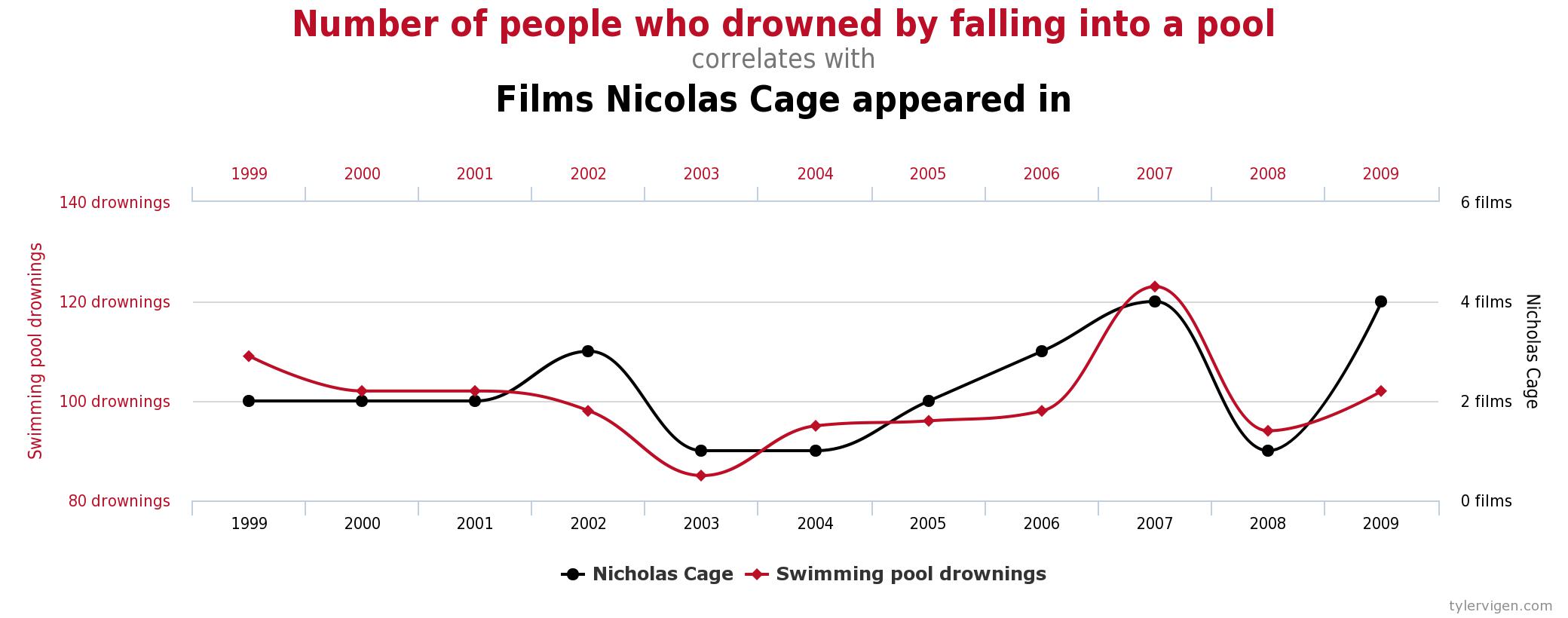
Association does not mean causation
Two variables are associated
(or related), if
the value of one variable gives you
information about the value of the other variable.
=> When comparing groups, this means that the proportions
or means take on different values in the different groups.
A confounding variable is a variable that is related both to the explanatory and to the response variable in such a way that its effects on the response variable cannot be separated from the effects of the explanatory variable.
Always think critically when you observe a cause-and-effect conclusion.
Association does not mean causation
Resampling confidence intervals
1- Draw a bootstrap sample from sample 1
2- Draw a bootstrap sample from sample 2
3- Compute your statistics (ex: relative risk of the conditional proportions) and store this value.
4- Repeat this process (steps 1-3) 10000 times
5- Determine the $\frac{\alpha}{2}$ and $(1-\frac{\alpha}{2})$ percentiles in your stored result array.