Analyzing more general situations
So far, we have explored tests of significance, confidence intervals, generalization, and causation for situations limited to the analysis of a single variable (categorical or quantitative), or to the comparison of two groups.
With linear regression, we've started to study more complex situations: the explanatory variable could actually get more than only two values, and we could make inference about an association of two quantitative variables.
Today, we will continue to study more general situations, and see how we can deal with situations in which we have to analyze more than two proportions.
Categorical variable(s)
We've came across the analysis of categorical variable(s), and we've seen that they can be presented/organized into contingency tables.
Single categorical variable
| Response variable |
|||
| Cat. #1 | |||
| Yes | 50 | ||
| No | 30 | ||
| Maybe | 20 | ||
Ex: Are the six colors of M&Ms equally likely in a pack?
Two categorical variables
| Response variable |
Explanatory variable | ||
| Cat. #1 | Cat. #2 | Cat. #3 | |
| Yes | 50 | 65 | 35 |
| No | 30 | 45 | 15 |
| Maybe | 20 | 10 | 10 |
Ex: Which treatment increases the survival rate of the patients?

Let's start with a simple example
Rock-Paper-Scissors (RPS) tournament
Let's consider that you want to enter a RPS competition (it does exist!), but you're looking to get an advantage and wonder if there is a pattern in the signs the other players tend to chose.
Do players equally use each hand sign? Or is one hand sign usually used more than the others?
Can we use statistics to help us win?

Rock Paper Scissors
A study analyzed the distribution of hand signs used by a group of students during a total of 381 games. The results are shown in the table below:
| Rock | Paper | Scissors | Total | |
| Observed count | 107 | 124 | 150 | 381 |
| Observed proportion | 0.281 | 0.325 | 0.394 | 1 |
Is the proportion of each signs equal?
What is the probability of observing such a distribution
of proportions if there were an equal chance for the 3 hand signs to be played?
Rock Paper Scissors
A study analyzed the distribution of hand signs used by a group of students during a total of 381 games. The results are shown in the table below:
| Rock | Paper | Scissors | Total | |
| Observed count | 107 | 124 | 150 | 381 |
| Observed proportion | 0.281 | 0.325 | 0.394 | 1 |
$H_0: \pi_\texclass{danger}{\mathrm{rock}} = \pi_\texclass{info}{\mathrm{paper}} = \pi_\texclass{warning}{\mathrm{scissor}}=\frac{1}{3}$
$H_a:$ at least one of the 3 $\pi_\mathrm{sign}$ is different from the others
The single categorical variable case
When we were studying the distribution of a single categorical variable with only two possible outcomes, we were comparing our observed proportion of success/failure to a null hypothesis (the value of the null hypothesis depends on the situation).
| Head | Tail | Total | |
| Observed count | 10 | 6 | 16 |
| Observed proportion | 0.625 | 0.375 | 1 |
$H_0: \texclass{danger}{\pi_\mathrm{head}}=\frac{1}{2}$

The single categorical variable case
When we were studying the distribution of a single categorical variable with only two possible outcomes, we were comparing our observed proportion of success/failure to a null hypothesis (the value of the null hypothesis depends on the situation).
| Correct | Incorrect | Total | |
| Observed count | 16 | 5 | 21 |
| Observed proportion | 0.76 | 0.24 | 1 |

$H_0: \texclass{warning}{\pi_\mathrm{correct}}=\frac{1}{3}$
Rock Paper Scissors
Could we apply the same strategy here?
Couldn't we just test independently $H_0: \pi_\mathrm{sign}=\frac{1}{3}$ for all three possible outcomes?
| Rock | Paper | Scissors | Total | |
| Observed count | 107 | 124 | 150 | 381 |
| Observed proportion | 0.281 | 0.325 | 0.394 | 1 |
No! The more inferences are made, the more likely erroneous inferences are to occur (multiple testing problem).
We want to compare our data to a single distribution pattern ($\frac{1}{3}/\frac{1}{3}/\frac{1}{3}$), so we need to find a way to perform the analysis in only one testing.
Rock Paper Scissors
Could we apply the same strategy here?
Couldn't we just test independently $H_0: \pi_\mathrm{sign}=\frac{1}{3}$ for all three possible outcomes?
| Rock | Paper | Scissors | Total | |
| Observed count | 107 | 124 | 150 | 381 |
| Observed proportion | 0.281 | 0.325 | 0.394 | 1 |
Comparing the distribution pattern of the three proportions to the theoretical distribution pattern:
How far the observed counts are from the expected (theoretical) counts if the null hypothesis ($\pi_\texclass{danger}{\mathrm{rock}} = \pi_\texclass{info}{\mathrm{paper}} = \pi_\texclass{warning}{\mathrm{scissor}}$) was true?
Expected counts
The expected counts are the amounts we should see in each category (cell) if the null hypothesis was true for that sample size.
For each cell, the expected count is the total sample size ($n_\mathrm{total}$) times the null proportion for each hand sign, $\pi_\mathrm{i}$.
| Rock | Paper | Scissors | Total | |
| Observed count | 107 | 124 | 150 | 381 |
| Observed proportion | 0.281 | 0.325 | 0.394 | 1 |
| Expected proportion | $\frac{1}{3}$ | $\frac{1}{3}$ | $\frac{1}{3}$ | 1 |
| Expected count | 127 | 127 | 127 | 381 |
Analyzing the expected counts
We have the observed and expected counts, now what could we do with these?
calculate the difference between observed and expected
| Rock | Paper | Scissors | |
| Observed | 107 | 124 | 150 |
| Expected | 127 | 127 | 127 |
How could we combine those 3 differences into a single statistic of interest? Add them up? Average them?
What could we do so we don't get a sum of zero?
Rock: $d_1 = 107-127=-20$
Paper: $d_2 = 124-127=-3$
Scissors: $d_3 = 150-127=23$
$\sum_{i=1}^3d_i=-20+(-3)+23=0$
Chi-squared ($\chi^2$) statistics
A statistic that is widely used to describe the difference in distribution patterns of categorical variable(s) is the square of the relative differences of each observed frequencies compared to the expected frequencies. This is known as the Chi-Squared statistic for comparing frequencies of a categorical variable.
$\chi^2$ summarizes the discrepancy between observed and expected frequencies:
- The smaller the overall discrepancy is between the observed and expected scores, the smaller the value of the $\chi^2$ will be.
- Conversely, the larger the discrepancy is between the observed and expected scores, the larger the value of the $\chi^2$ will be.
Does that remind you of anything?
It's kind of like calculating the residuals of a linear regression model but for an histogram (categories) instead!
How far is the observed distribution pattern of the observed frequencies from the theoretical distribution pattern?
$\chi^2$ goodness of fit test
When we calculate a $\chi^2$ statistic to compare distribution patterns of categorical variables, this is called a $\chi^2$ goodness of fit test.
| Rock | Paper | Scissors | |
| Observed | 107 | 124 | 150 |
| Expected | 127 | 127 | 127 |
$\chi^2=\frac{(107-127)^2}{127}+\frac{(124-127)^2}{127}+\frac{(150-127)^2}{127}$
$\chi^2=3.150+0.071+4.165$
$\chi^2=7.386$
What does a $\chi^2$ of 7.386 mean? Is it a large or a small value?
$\chi^2$ sampling distribution
What values of $\chi^2$ would we observe for a multitude of samples coming from the null distribution?
We need to compare the $\chi^2$ that we calculated to the distribution of this statistic assuming $H_0$ is true.
How do we get this?
- simulation
- theoretical distribution (requires validity conditions!)
Simulating the null hypothesis
For equally likely choices:
- Take 3 scraps of paper and label them Rock, Paper, Scissors. Fold or crumple them so they are indistinguishable
- Choose one at random and record the result. Repeat a number of times to match the original sample size and get a new table of observed counts.
- Calculate the $\chi^2$-statistic (compared to the expected counts).
- Repeat this many times (10000) to get a randomization distribution of many $\chi^2$-statistics under the assumption that the null hypothesis is true.
- How extreme is the actual test statistic in this randomization distribution? How many simulations ended up with a $\chi^2$ as extreme as the one you calculated from your original sample? (p-value)
Simulating the null hypothesis
Rock-Paper-Scissors $\chi^2$ randomization distribution
Note: $\chi^2$ will always be positive. Always use the right tail to find a p-value.
Observed $\chi^2$: 7.39
$\textrm{p-value} = 0.026$
We have strong evidence against the null hypothesis. At least one of the hand signs frequency can be considered statistically different to the expected frequency of this hand sign if the probability of choosing either hand sign was $\frac{1}{3}$.
Theory: $\chi^2$ distribution
If each of the expected counts are at least 10 (validity condition), AND if the null hypothesis is true, then the $\chi^2$ statistic follows a $\chi^2$–distribution, with degrees of freedom equal to:
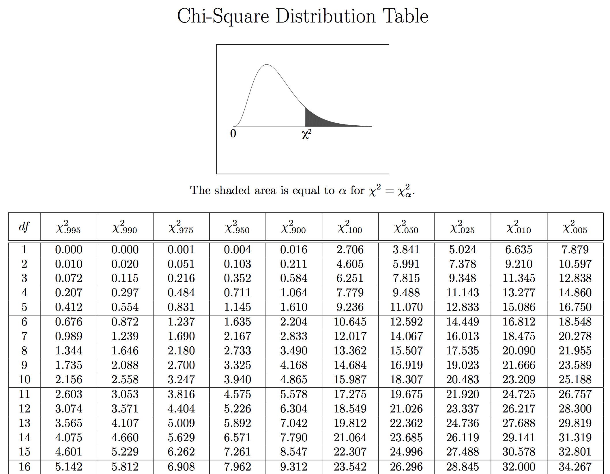

Theory: $\chi^2$ distribution
For Rock-Paper-Scissors:
df = 3 – 1 = 2
Simulation
Theoretical distribution
Follow up?
We found that there is a difference in distribution pattern that can be considered statistically significant (p-value<0.05) ... now what's next?
No standard approach to follow, there are many different follow-up approaches.
We want to know if one of the hand sign (rock, paper, scissors) is used more often compared to the others so we could play the opposite sign more often to get an advantage.
Now that we know that there is a statistical difference in the distribution pattern of the signs, we could use pairwise analysis of difference in proportions to determine exactly which signs are more often played.
Paper vs Scissors
$d=-0.068$
pvalue=0.0583
Paper vs Rock
$d=0.045$
pvalue=0.2058
Rock vs Scissors
$d=-0.113$
pvalue=0.0010
$\chi^2$ test for goodness of fit
A $\chi^2$ test for goodness-of-fit tests whether the distribution of a categorical variable is the same as some null hypothesized distribution.
Note that the null hypothesized proportions for each category do not have to be the same!
Ex: Are the six colors (green, orange, blue, red, yellow, brown) of M&Ms equally likely in a pack?
Does the grade distribution of the class follow the usual pattern?

$\chi^2$ test for goodness of fit
A $\chi^2$ test for goodness-of-fit tests whether the distribution of a categorical variable is the same as some null hypothesized distribution.
Exactly the same approach:
- State the null hypothesized proportions for each category, $\pi_i$. The alternative hypothesis is that at least one of the proportions is different from specified in the null.
- Calculate the expected counts for each cell as $n_\mathrm{total}\times\pi_i$.
- Calculate the $\chi^2$ statistic. $\chi^2=\sum_{i=1}^n\frac{(\mathrm{Observed}_i-\mathrm{Expected}_i)^2}{\mathrm{Expected}_i}$
- Simulate the null hypothesis and compute the p-value
- Interpret the p-value in context
Example of different expected $\pi_i$
In 1866, Gregor Mendel, the “father of genetics” published the results of his experiments on peas.
He found that his experimental distribution of peas closely matched the theoretical distribution predicted by his theory of genetics (involving alleles, and dominant and recessive genes)
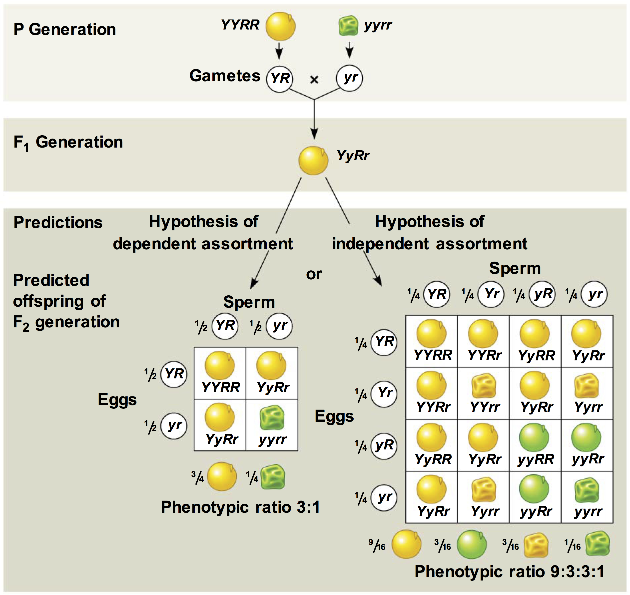
Mendel's pea experiment
Does the observed experimental distribution match the theoretical distribution predicted by genetics?
Let’s test these data against the null hypothesis of the proportions distribution based on the theory of genetics.
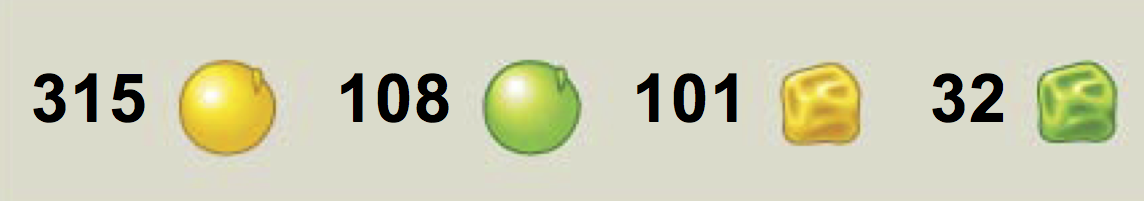
| Phenotype | Theoretical proportion | Observed count |
| Round, Yellow | $9/16$ | $315$ |
| Round, Green | $3/16$ | $108$ |
| Wrinkled, Yellow | $3/16$ | $101$ |
| Wrinkled, Green | $1/16$ | $32$ |
| Total | $1$ | $556$ |
Null Hypothesis:
$H_0: \pi_1=\frac{9}{16}, \pi_2=\frac{3}{16}, \pi_3=\frac{3}{16}, \pi_4=\frac{1}{16}$
Alternative Hypothesis:
$H_a:$ at least one $\pi_i$ is not as specified in $H_0$
Mendel's pea experiment
What is the expected count for each pea category? ($n_\mathrm{total}\times\pi_i$)
| Phenotype | Theoretical proportion | Observed count | Expected count |
| Round, Yellow | $9/16$ | $315$ | $556\times9/16=\texclass{warning}{312.75}$ |
| Round, Green | $3/16$ | $108$ | $556\times3/16=\texclass{warning}{104.25}$ |
| Wrinkled, Yellow | $3/16$ | $101$ | $556\times3/16=\texclass{warning}{104.25}$ |
| Wrinkled, Green | $1/16$ | $32$ | $556\times1/16=\texclass{warning}{34.75}$ |
| Total | $1$ | $556$ | $556$ |
What is the calculated $\chi^2$ from these results?
$\chi^2=\frac{(315-312.75)^2}{312.75}+\frac{(108-104.25)^2}{104.25}+\frac{(101-104.25)^2}{104.25}+\frac{(32-34.75)^2}{34.75}$
$\chi^2=0.016+0.135+0.101+0.218$
$\chi^2=0.470$
Mendel's pea experiment
Simulation
Theoretical distribution
Does this prove Mendel’s theory of genetics?
No! You should never accept the null hypothesis!!! A high p-value doesn’t “prove” or give evidence for anything. This p-value only suggests that the obtained distribution of pea phenotypes could have been observed if the null hypothesis was true.
$\chi^2$ test for association
The statistics behind a $\chi^2$ test easily extends to two categorical variables.
A $\chi^2$-test for association (often called a $\chi^2$-test for independence) tests for an association between two categorical variables.
Is soda preference associated with age?
| Soda | Age group | |||
| 15-25 | 26-40 | 41-55 | Total | |
| Coke | 54 | 45 | 69 | 168 |
| Pepsi | 19 | 41 | 38 | 98 |
| Sprite | 19 | 22 | 28 | 69 |
| Total | 92 | 108 | 135 | 335 |
Now we are interested to know if the proportions of preference for each soda is dependent of (associated to) the age group the person we asked the question to is in.
Is soda preference associated with age?
| Soda | Age group | |||
| 15-25 | 26-40 | 41-55 | Total | |
| Coke | 54 | 45 | 69 | 168 |
| Pepsi | 19 | 41 | 38 | 98 |
| Sprite | 19 | 22 | 28 | 69 |
| Total | 92 | 108 | 135 | 335 |
Null Hypothesis:
$H_0$: Soda preference is not associated with age
Alternative Hypothesis:
$H_a$: Soda preference is associated with age
Exemple for coke and age group (15-25):
$\mathrm{Expected}_\mathrm{coke}^\textrm{(15-25)}=\frac{168\times92}{335}=46.14$
Is soda preference associated with age?
| Soda | Age group | |||
| 15-25 | 26-40 | 41-55 | Total | |
| Coke | 54 | 45 | 69 | 168 |
| Pepsi | 19 | 41 | 38 | 98 |
| Sprite | 19 | 22 | 28 | 69 |
| Total | 92 | 108 | 135 | 335 |
| Soda | Age group | |||
| 15-25 | 26-40 | 41-55 | Total | |
| Coke | 46.14 | 54.16 | 67.7 | 168 |
| Pepsi | 26.91 | 31.59 | 39.49 | 98 |
| Sprite | 18.95 | 22.24 | 27.81 | 69 |
| Total | 92 | 108 | 135 | 335 |
Note: The expected counts maintain row and column totals, but redistribute the counts as if there were no association.
How do the observed results compared to the scenario of no-association?
compute the $\chi^2$ from all the cells in the table
Is soda preference associated with age?
| Soda | Age group | |||
| 15-25 | 26-40 | 41-55 | Total | |
| Coke | 54 | 45 | 69 | 168 |
| Pepsi | 19 | 41 | 38 | 98 |
| Sprite | 19 | 22 | 28 | 69 |
| Total | 92 | 108 | 135 | 335 |
| Soda | Age group | |||
| 15-25 | 26-40 | 41-55 | Total | |
| Coke | 46.14 | 54.16 | 67.7 | 168 |
| Pepsi | 26.91 | 31.59 | 39.49 | 98 |
| Sprite | 18.95 | 22.24 | 27.81 | 69 |
| Total | 92 | 108 | 135 | 335 |
$\chi^2=\frac{(54-46.14)^2}{46.14}+\frac{(45-54.16)^2}{54.16}+\frac{(69-67.7)^2}{67.7}+...+\frac{(22-22.24)^2}{22.24}+\frac{(28-27.81)^2}{27.81}$
$\chi^2=8.10$ Is it a big or low $\chi^2$?
We need the $\chi^2$ distribution
Simulating the null hypothesis
For no-association condition:
- Create an array for each of your explanatory variable categories (e.g.: age groups) with as many different outcomes as the response variable outcomes (e.g.: coke=0, pepsi=1, sprite=2)
- Pool together all the different arrays into a single population (if age doesn't influence soda choice, then all the age groups have the same probability of choosing one soda over another).
- Shuffle this population array (simulate the "no-association" condition).
- Split this array into groups of same group size as the original samples (each explanatory variable categories, age-groups), and calculate the new proportion you obtain for each of the soda.
- Calculate the $\chi^2$-statistic (compared to the expected counts).
- Repeat this many times (10000) to get a randomization distribution of many $\chi^2$-statistics under the assumption that the null hypothesis is true.
- Calculate the p-value (right tail only for $\chi^2$)
Theory
For a 2-ways contingency table, the number of degrees of freedom can be obtained by:
$df=(\textrm{Number of rows} − 1)\times(\textrm{Number of columns} − 1)$
For the soda study:
$df = (3-1)\times(3-1) = 4$
| Soda | Age group | |||
| 15-25 | 26-40 | 41-55 | Total | |
| Coke | 46.14 | 54.16 | 67.7 | 168 |
| Pepsi | 26.91 | 31.59 | 39.49 | 98 |
| Sprite | 18.95 | 22.24 | 27.81 | 69 |
| Total | 92 | 108 | 135 | 335 |
Is soda preference associated with age?
Simulation
Theoretical distribution
p-value > 0.05, we do not have strong evidence against the null hypothesis of no-association.
Soda preference does not seem to be associated with age.
Follow up
What if you find evidence of an association? How do we determine exactly where the association is?
Again, no standard approach to follow, several options are possible.
pairwise confidence intervals for the difference in proportions to determine exactly where the association lies.
Recap on $\chi^2$ tests
| $\chi^2$ for goodness of fit | $\chi^2$ test of independance |
| Test hypothesis about shape of discrete distribution | Test hypothesis about relationship of categorical variables |
| Are the frequencies I observe for my categorical variable consistent with my theory? | Are the two categorical variables associated with one another in the population? |
Goodness-of-fit test and test of intependence are in fact the same approach (how different are my data from the theoretical distribution?).
$\chi^2$ is just another statistic of interest, and the null randomization distribution can be easily simulated.
The theoretical approach to determine the $\chi^2$ distribution requires the use of the correct degrees of freedom number of the contingency table you are studying. Remember that you would also need a count>10 for all the cells as validity condition of the theoretical approach.