Last time: Correlation
Two quantitative variables association:
- Form? Linear
- Direction
- Strength
Correlation
($r$)
By analysing our sample, we are 95% confident that the true value of the correlation ($\rho$) between height and foot length is in the interval $(0.54, 0.86)$.
Going beyond correlation
If height and foot length are significantly correlated, couldn't we use the value of one of the variables to predict the value of the other one?
Could we use foot length to gain (unknown) information about someone height?
Why would we want to do that?
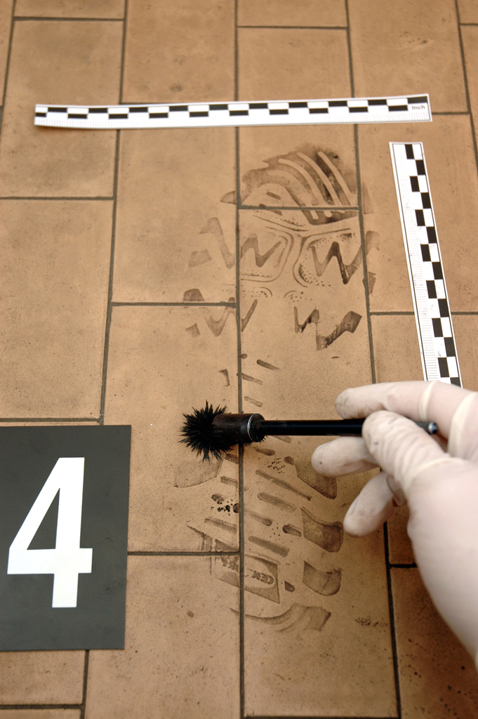
Forensic analysis:
Most people are not accustomed to looking at foot length, so describing the suspect as having a foot of 10.5inches long would probably not help find the suspect. It would be far more useful to tell people to look for a suspect who is of a certain height.
The accuracy of this prediction would depend on the size of the correlation between foot length and height

Anthropology:
Body proportions and the dimensions of various body segments,
including the long bones of their limbs and the bones of the
foot and hand have been used to estimate stature.
The accuracy of this prediction would depend on the size of the correlation between foot length and height
Going beyond correlation
Because the correlation coefficient only gives information about the direction and strength of an association, we cannot use it directly to get information of someone's height from his/her footprint.
If we decide the association is linear (strong $r$), it is useful to develop a mathematical model of that association.
The process of fitting a line to a set of data is called linear regression, and the line of best fit is called the regression line, which is the line that gets as close as possible to all of the data points.
We can use the regression line to give a predicted value of the response variable, based on a given value of the explanatory variable.
The regression line
Usually, rather than estimating predictions using a graph, we directly use the equation of the regression line.
Equation for a line:
$y= a + bx$
- $a$: y-intercept at $x=0$
- $b$: slope of the line (often called $m$)
Predicting the response variable from the explanatory
variable:
$\mathrm{Response}= a + b \times \mathrm{Explanatory}$
Notes on the regression line
When used to make prediction, the equation of the regression line is written:
- $x$: value of the explanatory variable
- $\overset{\hat{}}{y}$: predicted value of the response variable
For a given data set, the sign (positive, negative, or zero) for the correlation coefficient and the slope of the regression line must be the same.
The slope of the regression line can be interpreted as the predicted change in the average response variable for a one-unit change in the explanatory variable.
Linear regression is everywhere
Biology:
Colorimetric assay
Linear regression is everywhere
Biology:
Colorimetric assay
Physics:
Instrument calibration
Linear regression is everywhere
Biology:
Colorimetric assay
Physics:
Instrument calibration
Business:
Sale prediction, etc ...
Ice Cream
Linear regression is everywhere
Biology:
Colorimetric assay
Physics:
Instrument calibration
Business:
Sale prediction, etc ...
How does linear regression work?
The vertical distance from a data point to the regression
line is called a residual.
$\mathrm{Residual} = \mathrm{Observed} − \mathrm{Predicted}$
$\mathrm{Residual} = y − \overset{\hat{}}{y}$
- Points above the line positive residuals
- Points below the line negative residuals.
- If the predicted values closely match the observed data values, the residuals will be small.
How does linear regression work?
- Points above the line positive residuals
- Points below the line negative residuals.
- If the predicted values closely match the observed data values, the residuals will be small.
How does linear regression work?
The line that fits the data best is the one where the residuals are close to zero.
Instead of working directly with the residuals, we usually try to minimize the sum of the square of the residuals:
$SS_{residuals}=\sum_{i=1}^{n}(y_i-\overset{\hat{}}{y_i})^2$
Notes on minimizing the $SS_{residuals}$
The errors (residuals) are squared to remove the $+$ or $-$ signs and prevent the positive and negative errors to cancel out each others, which could give you a value of zero.
Most statistical software packages use a procedure called Ordinary Least Squares (OLS) to find the line of best fit. This procedure finds a line that minimizes the sum of the squared errors.
While OLS is pretty much the standard, different penalty functions can be use as well. For example, the Median Absolute Deviation (MAD) uses the absolute error, and so will be more robust to outliers since it assigns less weight to outliers than OLS.
How does linear regression work?
Linear regression analysis
Linear regression analysis consists of more than just fitting a linear line through a cloud of data points. The linear regression analysis of a dataset can be decomposed in 3 stages:
- Analyzing the correlation and directionality of the data (checking if linear regression is an appropriate model for the data you want to analyze)
- Estimating the model using the data (fitting the line, estimating the best parameters for the line equation)
- Evaluating the validity and usefulness of the model
Evaluating the model
Three statistics are commonly used in linear regression analysis to evaluate how well the model fit the data:
- The $R^2$, or coefficient of determination
- The $RMSE$, or Root Mean Square Error
- The $F$-statistic (we will talk about it later in class, when we will compare more than two quantitative variables)
All three statistics are based on two sums of squares:
| Total Sum of Squares ($TSS$) | Sum of Squares Error ($SSE$) |
| it measures how far the response variable data are from the mean. $TSS=\sum_{i=1}^{n}(y-\texclass{info}{\bar{y}})^2$ | it measures how far the data are from the model’s predicted values. $SSE=\sum_{i=1}^{n}(y-\texclass{danger}{\overset{\hat{}}{y}})^2$ |
Different combinations of these two values provide different information about how the regression model compares to the mean model.
Coefficient of determination, $R^2$
$R^2$ measures the percentage of total variation in the response variable that is explained by the linear relationship.
$R^2=1-\frac{\textrm{Sum of squared errors (SSE)}}{\textrm{Total sum of squares (TSS)}}$ $= 1-\frac{\sum_{i=1}^{n}(y-\texclass{danger}{\overset{\hat{}}{y}})^2}{\sum_{i=1}^{n}(y-\texclass{info}{\bar{y}})^2}$$
Notes:
- Another way to compute $R^2$ is by litteraly calculating the square of the correlation coefficient ($r$). $R^2 = r^2$
- The slope ($m$) of the regresion line tells you how much change in $Y$ you can expect based on a given change in $X$. The coefficient $R^2$ tells you how much of the variation in $Y$ is attributable to (explained by) the variation in $X$. The rest of the variation (or “noise”), is accounted by other factors, such as measurement error, individual variation, etc.
Root mean square error, $RMSE$
The $RMSE$ measures how close the observed data points are to the model’s predicted values.
The $RMSE$ is a common metric to evaluate model performance and computes the square root of the average squared residual (distance from the prediction to the best fit).
$RMSE=\sqrt{\frac{1}{n}\sum_{i=1}^{n}(y-\overset{\hat{}}{y})^2}$
The key idea behind the computation of the $RMSE$ is that predictions ($\overset{\hat{}}{y}$) that are far away from the true observed data value ($y$) will contribute more heavily to increasing the value of the $RMSE$ than predictions that are close to the true values.
Lower values of RMSE indicate better fit.
Model evaluation, $R^2$ vs $RMSE$
| $R^2$ | $RMSE$ |
| Square of the correlation coefficient | Square root of the average squared residual |
| Both give an indication about the "goodness of the fit" | |
| $R^2$ is conveniently scaled between 0 and 1 (relative measure of fit) | $RMSE$ is not scaled to any particular value (absolute measure of fit) |
| $R^2$ can be more easily interpreted in the context of the linear association analyzed (how successful the fit is in explaining the variation of the data) | $RMSE$ explicitly provides information about how much our predictions deviate, on average, from the actual values in the dataset |
| Its main purpose is either the prediction of future outcomes or the testing of hypotheses. | It is one of the most important criterion for fit if the main purpose of the model is prediction |
The use of linear regression analysis
There are 3 major uses for regression analysis:
Causal analysis: it might be used to identify the strength of the effect that the independent variable(s) have on a dependent variable. Typical questions are what is the strength of relationship between dose and effect, sales and marketing spend, age and income, etc...
Forecasting: it can be used to forecast effects or impacts of changes. That is regression analysis helps us to understand how much will the dependent variable change, when we change one or more independent variables. Typical questions are how much additional $Y$ would I get for one additional unit $X$.
Prediction: it can be used to predict trends and future values. The regression analysis can be used to get point estimates. Typical questions are what will the price for gold be in 6 month from now? What is the total effort for a task X?
Regression caution #1
Extrapolation: The regression line should only be used to predict values within or close to those contained in the dataset. Far beyond the dataset, the trend may change and the predictions will be incorrect.

Nature 431, 525 (30 September 2004)
Regression caution #1
Extrapolation: The regression line should only be used to predict values within or close to those contained in the dataset. Far beyond the dataset, the trend may change and the predictions will be incorrect.

Nature 431, 525 (30 September 2004)
Regression caution #1
Extrapolation: The regression line should only be used to predict values within or close to those contained in the dataset. Far beyond the dataset, the trend may change and the predictions will be incorrect.
| Year | Predicted | Real |
| 2008 | 10.57 | 10.78 |
| 2012 | 10.50 | 10.75 |
| 2016 | 10.43 | 10.71 |
| Year | Predicted | Real |
| 2008 | 9.73 | 9.69 |
| 2012 | 9.68 | 9.63 |
| 2016 | 9.64 | 9.81 |
Regression caution #1
Extrapolation: The regression line should only be used to predict values within or close to those contained in the dataset. Far beyond the dataset, the trend may change and the predictions will be incorrect.
"A. J. Tatem and colleagues calculate that women may out-sprint men by the middle of the twenty-second century.
They omit to mention, however, that (according to their analysis) a far more interesting race should occur in about 2636, when times of less than zero seconds will be recorded."
-- Kenneth Rice (2004) --
Regression caution #2
Generalization: A regression model developed from a specific dataset should not be used to generalize about observational units not related to the original dataset or to conclude about the general pattern of the phenomena.
If you develop a linear model from data collected on a specific sport team in order to predict how this team will perform in the near future, it is unlikely that the same model would be able to accurately predict how all the other teams will perform. Although we may find some kind of relationship between the variable recorded on the team we are studying, the same relationships might not exist for another team.
Regression caution #3
Causation: Although we imply a causal relationship when we use linear regression, regression analysis will not prove causality between two variables.
Recall that linear regression is a procedure strictly numeric; you may find that two totally unrelated variables give a significant $R^2$.
When studying a phenomena, you must understand the phenomena being researched and the regression procedure in order to interpret the results appropriately.
Regression caution #4
Validity: Plot the data! Although the regression line can be calculated for any set of paired quantitative variables, it is only appropriate to use a regression line when there is a linear trend in the data.
| Set #1 | Set #2 | Set #3 | Set #4 | ||||
|---|---|---|---|---|---|---|---|
| x | y | x | y | x | y | x | y |
| 10 | 8.04 | 10 | 9.14 | 10 | 7.46 | 8 | 6.58 |
| 8 | 6.95 | 8 | 8.14 | 8 | 6.77 | 8 | 5.76 |
| 13 | 7.58 | 13 | 8.74 | 13 | 12.74 | 8 | 7.71 |
| 9 | 8.81 | 9 | 8.77 | 9 | 7.11 | 8 | 8.84 |
| 11 | 8.33 | 11 | 9.26 | 11 | 7.81 | 8 | 8.47 |
| 14 | 9.96 | 14 | 8.1 | 14 | 8.84 | 8 | 7.04 |
| 6 | 7.24 | 6 | 6.13 | 6 | 6.08 | 8 | 5.25 |
| 4 | 4.26 | 4 | 3.1 | 4 | 5.39 | 19 | 12.5 |
| 12 | 10.84 | 12 | 9.13 | 12 | 8.15 | 8 | 5.56 |
| 7 | 4.82 | 7 | 7.26 | 7 | 6.42 | 8 | 7.91 |
| 5 | 5.68 | 5 | 4.74 | 5 | 5.73 | 8 | 6.89 |
| Correlation | 0.86 |
| Regression line | y = 3 + 0.5x |
Regression caution #5
Resistance: Outliers can have a strong influence on the regression line (similarly to what we saw for correlation). Lots of robust linear regression algorithms are capable of dealing with outliers by giving them less weight in the residual minimization function.
In particular, data points for which the explanatory value (x) is an outlier are often called influential points because they exert an overly strong effect on the regression line.

Interpreting the residuals plot
A value much lower or much larger than the other ones in the residual plot might
be the sign of the presence of an outlier in the dataset,
that may reduce the strength of the regression model
(large error = lower $R^2$).
Depending of your study, you may decide to use a robust linear regression method.
Interpreting the residuals plot
A residual lying at the far end of the
plot, directly on the $0$ line is the sign of an
outlier that has pulled the regression line towards it.
This type of outlier "artificially" increases
the $R^2$, (this outlier has no error because the line has passed right through it).
The equation and predictions from the obtained regression
line are likely to be incorrect.
Interpreting the residuals plot
A fan shape in the residuals plot indicates that the
amount of error is not constant along the regression line. At the lower end of the line, the errors are small; at the high end, the errors are large.
You often encounter this kind of heteroscedasticity (hetero = different, scedastic = scatter) when an
additional variable is influencing the relationship.
Interpreting the residuals plot
Residuals in a curve indicate that the relationship between the two variables is not linear.
You need to reconsider your variables or conduct non-linear regression analysis (not covered in this class).